VAEs and GANs: Two Ways to Sample What You Can't Write Down

A language model generates by writing its distribution down: the chain rule splits $p(x)$ into one next-token distribution after another (What “Generative” Means), each a softmax that is cheap to compute and sample from. The chain rule works for any data, images included, and autoregressive image models exist (PixelCNN, ImageGPT). But a 512×512 color image is 786,432 numbers, which means 786,432 sequential steps in a pixel order that nothing about the picture picks out. So generative models for images mostly took two other routes, both built on the same idea: start from simple noise $z$, and learn a network that maps it to data.

• The variational autoencoder (VAE) keeps a likelihood, but can’t compute it exactly, so it maximizes a lower bound, with an encoder to make the bound tight.
• The generative adversarial network (GAN) gives up on likelihood altogether: a second network, the critic, learns to tell real data from generated, and the generator learns to fool it.

The choice shows up in what goes wrong. VAEs put samples where there is no data; GANs drop modes, and sometimes fail to train at all. This post derives both, checks the math numerically, and trains a VAE, a GAN and one improved GAN (WGAN-GP) on the same small test where each failure is visible.

Table of contents

Latent variables

A latent-variable model says each data point $x$ was made from a hidden code $z$: draw $z$ from a simple prior $p(z)$, usually $\mathcal N(0, I)$, then draw $x$ from $p_\theta(x \mid z)$, a distribution whose parameters a neural network (the decoder) computes from $z$. Sampling is easy, two steps. The likelihood of a data point is not:

an integral over every code that could have produced $x$. With a neural decoder it has no closed form, and estimating it by sampling $z$ from the prior fails because almost no random code produces any particular $x$. Both models below are ways of training $\theta$ without ever computing this integral.

An ordinary autoencoder has the pieces but not the probability: an encoder squeezes $x$ into a code, a decoder rebuilds $x$ from it, and the two train to make the reconstruction match. Its codes land wherever training puts them, so a random point in code space usually decodes to nothing useful, and there is no way to sample from it. The VAE fixes exactly that.

The ELBO, derived

Give the model an encoder $q_\phi(z \mid x)$: a network that, for each $x$, outputs a distribution over the codes that could have made it. Multiply and divide by it inside the integral, and the likelihood becomes an expectation under $q$:

The inequality is Jensen’s ($\log$ is concave, so the log of an average is at least the average of the logs). Splitting the right side gives the evidence lower bound (ELBO):

The first term rewards codes that decode back to $x$: it is the autoencoder’s reconstruction loss. With a Gaussian decoder of fixed variance $s^2$ it is minus the squared error divided by $2s^2$, plus a constant. The second term is the KL divergence from Cross-Entropy and the Softmax Gradient, and it is what makes sampling work: it pulls every encoding toward $\mathcal N(0, I)$, so the region the prior draws from is the region the decoder was trained on.

How loose is the bound? Bayes’ rule says $p_\theta(x \mid z)\, p(z) = p_\theta(z \mid x)\, p_\theta(x)$, so the quantity inside the ELBO’s expectation is $\log p_\theta(x) - \log \big(q_\phi(z \mid x) / p_\theta(z \mid x)\big)$. The first part doesn’t depend on $z$; the second, averaged over $q$, is a KL divergence. So the gap is exactly:

The ELBO is the log-likelihood minus how far the encoder is from the true posterior. Since $\log p_\theta(x)$ doesn’t depend on $\phi$, maximizing the ELBO over $\phi$ only shrinks that gap: it makes the encoder a better posterior. Maximizing over $\theta$ can do either of two things: raise $\log p_\theta(x)$, or move the model’s true posterior toward whatever the encoder outputs, which shrinks the gap without improving the model.

The second option has a known failure. If the decoder is powerful enough to model $x$ without looking at $z$ (an autoregressive decoder for text, say), the cheapest way to raise the ELBO is to ignore $z$ altogether: the encoder outputs the prior for every input, the KL term drops to zero, and the codes carry no information. This is posterior collapse. A related knob is the weight on the KL term, written $\beta$ (the $\beta$-VAE, Higgins et al., 2017): $\beta > 1$ pushes codes harder toward the prior and $\beta < 1$ favors reconstruction. At $\beta < 1$ the objective is no longer a bound on $\log p(x)$; at $\beta > 1$ it is a looser one.

Checking the bound exactly

With a linear decoder, $p(x \mid z) = \mathcal N(Wz + b,\ s^2 I)$, everything has a closed form: $p(x)$ is Gaussian with covariance $WW^\top + s^2 I$, and so is the posterior. That makes the identity above checkable, in 2-D. elbo_check.py sets up the model, its exact $\log p(x)$ and its true posterior; the ELBO and the check for four choices of $q$ are:

def elbo(mu, sigma, n=200_000):
    """Reconstruction term by sampling (the reparameterization trick: z = mu +
    sigma * eps), KL to the prior in closed form."""
    z = mu + sigma * rng.standard_normal((n, 2))
    r = x - z @ W.T - b
    rec = (-0.5 * (r ** 2).sum(1) / s ** 2 - np.log(2 * np.pi * s ** 2)).mean()
    kl = 0.5 * (mu ** 2 + sigma ** 2 - 1 - np.log(sigma ** 2)).sum()
    r0 = x - W @ mu - b                               # the same expectation, in closed form
    exact = -0.5 * (r0 @ r0 + (W ** 2 * sigma ** 2).sum()) / s ** 2 - np.log(2 * np.pi * s ** 2)
    return rec, exact, kl

log_px = log_normal(x, b, W @ W.T + s ** 2 * np.eye(2))
P = np.linalg.inv(np.eye(2) + W.T @ W / s ** 2)      # posterior covariance
m = P @ W.T @ (x - b) / s ** 2                        # posterior mean
print(f"log p(x), exact: {log_px:.4f}")
print(f"true posterior: mean ({m[0]:.3f}, {m[1]:.3f}), "
      f"std ({np.sqrt(P[0, 0]):.3f}, {np.sqrt(P[1, 1]):.3f}), correlation {P[0, 1] / np.sqrt(P[0, 0] * P[1, 1]):.3f}\n")
print(f"{'q(z|x)':36s} {'recon (sampled, exact)':>22s} {'KL to prior':>11s} {'ELBO':>8s} {'gap':>7s} {'KL to post':>10s}")
# The best diagonal q (smallest KL to the posterior) keeps the posterior's
# mean but takes std_j = 1 / sqrt(precision_jj), not the posterior's own
# marginal stds: Kingma and Welling's encoder can't do better than this.
best = 1 / np.sqrt(np.diag(np.linalg.inv(P)))
cases = [("best diagonal Gaussian", m, best),
         ("posterior's mean and marginal stds", m, np.sqrt(np.diag(P))),
         ("right mean, stds 3x too wide", m, 3 * np.sqrt(np.diag(P))),
         ("the prior, N(0, I)", np.zeros(2), np.ones(2))]
for name, mu, sigma in cases:
    rec, exact, kl = elbo(mu, sigma)
    print(f"{name:36s} {rec:10.4f} {exact:10.4f}  {kl:11.4f} {exact - kl:8.4f} {log_px - (exact - kl):7.4f} "
          f"{kl_gauss(mu, np.diag(sigma ** 2), m, P):10.4f}")

Full script: elbo_check.py

log p(x), exact: -2.3429
true posterior: mean (0.365, 0.618), std (0.442, 0.479), correlation -0.210

q(z|x)                               recon (sampled, exact) KL to prior     ELBO     gap KL to post
best diagonal Gaussian                  -1.3081    -1.3066       1.0590  -2.3655  0.0226     0.0226
posterior's mean and marginal stds      -1.3417    -1.3435       1.0231  -2.3666  0.0237     0.0237
right mean, stds 3x too wide            -8.0050    -8.0153       0.5245  -8.5398  6.1969     6.1969
the prior, N(0, I)                      -6.1847    -6.1916       0.0000  -6.1916  3.8487     3.8487

KL(N(mu, sigma^2) || N(0, I)) for mu = (1, -0.5), sigma = (0.5, 2): 1.7500 nats

Four encoders for the same $x$, and in each the gap between $\log p(x)$ and the ELBO equals the KL from $q$ to the true posterior, to four decimals. (The ELBO column uses the closed-form reconstruction term; the sampled one agrees with it to about 0.01, which is the Monte Carlo noise a VAE trains with.)

The first two rows are the instructive ones. The true posterior’s two coordinates are correlated ($-0.21$), and a VAE encoder that outputs a mean and one standard deviation per coordinate (a diagonal Gaussian, the usual choice) can’t represent that. The best it can do is the first row, 0.0226 nats short of $\log p(x)$, which for two coordinates with correlation $\rho$ is $-\tfrac12 \log(1 - \rho^2)$. That shortfall, from restricting $q$ to a simple family, is the approximation gap. Note that the best diagonal $q$ isn’t the one that copies the posterior’s own standard deviations (second row, 0.0237): minimizing $\operatorname{KL}(q \,\|\, p)$ makes $q$ narrower than the posterior’s marginals, a general habit of this direction of KL. Making the stds three times too wide costs 6.2 nats; using the prior as the encoder, ignoring $x$ entirely, costs 3.8.

The KL term, worked

For a diagonal Gaussian encoder, $q = \mathcal N(\mu, \operatorname{diag}\sigma^2)$, against the prior $\mathcal N(0, I)$, the KL needs no sampling, and it splits into a sum over coordinates:

Take $\mu = (1, -0.5)$ and $\sigma = (0.5, 2)$. The first coordinate gives $1 + 0.25 - 1 - \log 0.25 = 0.25 + 1.386 = 1.636$; the second gives $0.25 + 4 - 1 - \log 4 = 3.25 - 1.386 = 1.864$. Half their sum is 1.75 nats, the last line of the output above. Each part of the formula has a job: $\mu_j^2$ charges for moving away from the origin, and $\sigma_j^2 - 1 - \log \sigma_j^2$, which is zero at $\sigma_j = 1$ and positive on both sides, charges for being narrower or wider than the prior. A code that shrinks to a point to reconstruct perfectly pays $-\log \sigma_j^2 \to \infty$, which is what keeps the codes spread out enough to sample from.

The reparameterization trick

The reconstruction term is an expectation over $z \sim q_\phi(z \mid x)$, and training needs its gradient with respect to $\phi$. But $\phi$ sits in the distribution the expectation is taken over, not in the thing being averaged, so averaging the gradient of samples doesn’t work: a sampled $z$ carries no record of how it depended on $\phi$. The fix is to move the randomness outside the network:

Now $z$ is an ordinary differentiable function of $\phi$, with $\varepsilon$ an input like any other, and backpropagation (Backpropagation, by Hand) flows through the sample. One draw of $\varepsilon$ per example gives an unbiased gradient estimate, usually with far less variance than the score-function estimator that policy gradients use (Reinforcement Learning for Language Models), which needs only $\nabla_\phi \log q$, not a path through the sample, and so works for discrete choices where this trick can’t. That one line, published at the same time by Kingma and Welling (2013) and by Rezende, Mohamed and Wierstra (2014), is what made VAEs train with plain SGD. It appears in the experiment below as z = mu + torch.randn_like(mu) * (0.5 * logvar).exp().

GANs: learn a critic instead

A GAN keeps the generator, $x = G(z)$ with $z \sim \mathcal N(0, I)$, and drops the likelihood and the encoder. In their place is a discriminator $D(x) \in (0, 1)$, trained to output the probability that $x$ is real. The two play a minimax game (Goodfellow et al., 2014):

For $D$ this is just binary cross-entropy on real versus generated. Fix the generator, whose samples follow some distribution $q$, and the best discriminator can be found pointwise: maximizing $p \log D + q \log(1-D)$ over $D$ at each $x$ gives

Put it back into $V$ and the value is a known divergence:

where the Jensen-Shannon divergence $\operatorname{JS}$ is the average KL from $p$ and from $q$ to their mixture $m = (p+q)/2$. So against a perfect critic, the generator minimizes the JS divergence to the data, reaching $-\log 4$ exactly when $q = p$. The experiment script, gen2d.py, checks the identity on two 1-D Gaussians a distance 1.5 apart, by integrating on a grid:

# The GAN's value at the optimal discriminator is 2 JS(p, q) - log 4: checked
# for two 1-D Gaussians on a grid.
xs = np.linspace(-10, 10, 20001); dx = xs[1] - xs[0]
p = np.exp(-0.5 * xs ** 2) / math.sqrt(2 * math.pi); q = np.exp(-0.5 * (xs - 1.5) ** 2) / math.sqrt(2 * math.pi)
Dstar = p / (p + q)
value = (p * np.log(Dstar) + q * np.log(1 - Dstar)).sum() * dx
m = (p + q) / 2
js = 0.5 * ((p * np.log(p / m)).sum() + (q * np.log(q / m)).sum()) * dx
print(f"optimal-discriminator value {value:.4f}; 2 JS - log 4 = {2 * js - math.log(4):.4f}")

Full script: gen2d.py

optimal-discriminator value -0.9440; 2 JS - log 4 = -0.9440

Why GANs are hard to train

The derivation assumes a perfect critic and smooth distributions; training has neither, and three problems follow.

• Saturation. Early on, generated samples are easy to spot, so $D(G(z)) \approx 0$ and $\log(1 - D(G(z)))$ is flat: the generator gets almost no gradient. The fix from the original paper, used ever since, is the non-saturating loss: train $G$ to maximize $\log D(G(z))$ instead, which has the same fixed point and a strong gradient exactly when the generator is losing. It does change what is minimized: against the optimal discriminator it works out to $\operatorname{KL}(q \,\|\, p) - 2\,\operatorname{JS}(p \,\|\, q)$ (Arjovsky and Bottou, 2017). That reverse KL charges heavily for samples where there’s no data, and almost nothing for data the generator never produces: one reason GANs drop modes.
• Disjoint supports. By the manifold hypothesis, real images lie near a thin, low-dimensional surface in pixel space, and generated ones lie on the image of a low-dimensional $z$. Two such surfaces generally meet only in a set of volume zero, and then JS sits at its maximum, $\log 2$, however close the surfaces are: its gradient is zero, and nothing says “move this way.”
• Mode collapse. Nothing in the game rewards covering all the data. A generator that produces a few convincing kinds of output can win each round; the critic learns to reject them, the generator jumps to other ones, and the pair can cycle instead of converging.

Wasserstein GANs (Arjovsky et al., 2017) attack the second problem by changing the distance. The Wasserstein-1 (earth-mover’s) distance is the least average distance mass has to move to turn $q$ into $p$, and it keeps shrinking smoothly as two distributions approach, overlapping or not. By a duality theorem it equals the largest gap $\mathbb E_p[f(x)] - \mathbb E_q[f(x)]$ over all functions $f$ with slope at most 1 everywhere (1-Lipschitz). So the critic becomes $f$, outputs any real number, and maximizes that gap; the generator minimizes it. Enforcing the slope limit is the hard part. The original paper clipped weights; WGAN-GP (Gulrajani et al., 2017) instead penalizes the critic’s gradient norm for straying from 1 at random points between real and generated samples, and trains the critic several steps per generator step (five, in the paper and below).

Three models, one test

The standard test for all of this is small: eight Gaussian blobs on a ring of radius 2, each with standard deviation 0.05. Collapse is easy to see in 2-D, and two numbers measure it from 2,000 samples: modes covered (a mode counts if more than 1% of samples, over 20 of the 2,000, land within 3 standard deviations of it) and share near a mode (the fraction of samples within 3 standard deviations of any mode). They are toy versions of the two halves of every generative metric: recall, how much of the data the model can produce, and precision, how much of what it produces looks like data. On images the standard single number is the Fréchet Inception Distance (FID), which compares the mean and covariance of real and generated images’ features in a pretrained classifier, and mixes both halves; precision and recall measured separately in the same feature space (Kynkäänniemi et al., 2019) keep them apart.

The same MLP size for every network, 6,000 generator steps, three seeds each. Two settings to flag: the VAE’s decoder noise is set to 0.05, the data’s own spread, which I could only choose because I made the data; and WGAN-GP gets five critic steps per generator step at half the learning rate (with Adam’s $\beta_1 = 0.5$ for both GANs, where the WGAN-GP paper used 0), so equal generator steps are not equal compute. The script is gen2d.py. Besides the two trainers below, it holds the data, the scoring and the check of the discriminator’s value, and the two later scripts load it by that name. It runs on the CPU; on an Apple M4 laptop this post’s code takes about 3 minutes in all. The two trainers:

def vae(seed, steps=6000, beta=1.0):
    """Encoder gives q(z|x) = N(mu, sigma^2) in 2-D; decoder gives p(x|z) =
    N(f(z), 0.05^2 I). Loss: minus the ELBO = reconstruction + KL to N(0, I)."""
    g = torch.Generator().manual_seed(seed); torch.manual_seed(seed)
    enc, dec = mlp(2, 4), mlp(2, 2)
    opt = torch.optim.Adam([*enc.parameters(), *dec.parameters()], 1e-3)
    for _ in range(steps):
        x = data(256, g)
        mu, logvar = enc(x).chunk(2, -1)
        z = mu + torch.randn_like(mu) * (0.5 * logvar).exp()            # the reparameterization trick
        rec = ((dec(z) - x) ** 2).sum(-1) / (2 * 0.05 ** 2)
        kl = 0.5 * (mu ** 2 + logvar.exp() - 1 - logvar).sum(-1)
        loss = (rec + beta * kl).mean()
        opt.zero_grad(); loss.backward(); opt.step()
    with torch.no_grad():
        return score(dec(torch.randn(2000, 2)))

def gan(seed, steps=6000, wgan=False):
    """Generator maps 2-D noise to points; the critic tells data from
    samples. Ordinary GAN: the non-saturating loss of Goodfellow et al.
    WGAN-GP: a critic score difference with a gradient penalty."""
    g = torch.Generator().manual_seed(seed); torch.manual_seed(seed)
    G, D = mlp(2, 2), mlp(2, 1)
    og = torch.optim.Adam(G.parameters(), 1e-4 if wgan else 2e-4, betas=(0.5, 0.9))
    od = torch.optim.Adam(D.parameters(), 1e-4 if wgan else 2e-4, betas=(0.5, 0.9))
    bce = nn.BCEWithLogitsLoss()
    for step in range(steps):
        for _ in range(5 if wgan else 1):
            x, fake = data(256, g), G(torch.randn(256, 2)).detach()
            if wgan:
                eps = torch.rand(256, 1)
                mix = (eps * x + (1 - eps) * fake).requires_grad_(True)
                grad = torch.autograd.grad(D(mix).sum(), mix, create_graph=True)[0]
                ld = D(fake).mean() - D(x).mean() + 10 * ((grad.norm(dim=1) - 1) ** 2).mean()
            else:
                ld = bce(D(x), torch.ones(256, 1)) + bce(D(fake), torch.zeros(256, 1))
            od.zero_grad(); ld.backward(); od.step()
        fake = G(torch.randn(256, 2))
        lg = -D(fake).mean() if wgan else bce(D(fake), torch.ones(256, 1))
        og.zero_grad(); lg.backward(); og.step()
    with torch.no_grad():
        return score(G(torch.randn(2000, 2)))

Full script: gen2d.py

model                    modes covered (of 8), per seed   share of samples near a mode
VAE                                 8  8  8            52%  48%  51%
GAN (non-saturating)                8  7  8            89%  82%  88%
WGAN-GP                             8  8  1            72%  65%  2%

The same M4 trainings drawn, for the four runs that show the differences (1,000 of each run’s 2,000 samples; the circles are the 3-standard-deviation region around each true mode; points outside the square are not drawn, and only WGAN-GP seed 2 has any):

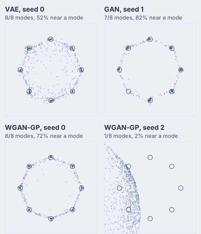
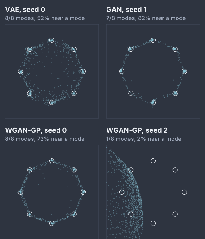
The VAE puts samples where there’s no data. It covers all eight modes in every seed, because the reconstruction term punishes any training point it can’t rebuild: dropping a mode is expensive. But only about half its samples land on a mode; most of the rest sit along the ring between modes, and a few inside it. The textbook explanation is averaging: if neighboring modes’ codes overlap, the decoder’s best guess under squared error is a point between them. That predicts that even reconstructions would blur, and it can be tested, by decoding three kinds of code from the same trained models:

import torch
# Where do the VAE's off-mode samples come from? gen2d.py's vae(), trained
# the same way, but returning the encoder and decoder instead of a score.
src = open("gen2d.py").read().split("# The GAN's value")[0]
ns = {}; exec(src.replace("return score(dec(torch.randn(2000, 2)))", "return enc, dec"), ns)
print(f"{'seed':>4s} {'reconstructions':>16s} {'z from the encoders':>20s} {'z from the prior':>17s}")
for seed in range(3):
    enc, dec = ns["vae"](seed)
    with torch.no_grad():
        x = ns["data"](2000, torch.Generator().manual_seed(99))
        mu, logvar = enc(x).chunk(2, -1)
        rec = dec(mu)                                                    # decode each point's mean code
        agg = dec(mu + torch.randn_like(mu) * (0.5 * logvar).exp())      # a code the encoder could give
        prior = dec(torch.randn(2000, 2))                                # what sampling the VAE does
    print(f"{seed:4d} " + "".join(f"{ns['score'](v)[1]:>{w}.0%}" for v, w in ((rec, 16), (agg, 21), (prior, 18))), flush=True)

Full script: vae_codes.py

seed  reconstructions  z from the encoders  z from the prior
   0             100%                 100%               52%
   1             100%                  99%               50%
   2             100%                 100%               48%

Averaging is not what happens here. Every reconstruction lands on its mode, and so do 99–100% of codes drawn from the encoders’ own distributions. Only codes drawn from the prior go wrong. The encoders together use only part of the prior’s space (the aggregate posterior, the mix of all the $q(z \mid x)$, doesn’t fill $\mathcal N(0, I)$), and a prior sample that falls in a gap between the regions they use decodes to whatever the continuous decoder passes through on its way from one mode to the next: a point on the ring between them. The KL term pulls each $q(z \mid x)$ toward the prior but can’t close those gaps. On images both causes are at work: decoders do average when a code is ambiguous, which gives the familiar blur, and prior samples from the gaps give implausible images. Later fixes target the gap: a learned prior, or a second model that samples from the aggregate posterior, which is what latent diffusion amounts to.

The GAN is sharp and can drop modes. In the run above, 82–89% of its samples land on a mode, because the critic rejects anything off the data, and an in-between sample is the easiest thing for it to spot. But nothing makes it cover them all: in seed 1 the lower-left mode fell below the 1% threshold, with only a few stray samples near it. On a rerun on an NVIDIA RTX 3090 (its saved outputs), all three seeds kept every mode, and seed 1 put only 53% of its samples near one, against 88–89% for the other two. A generator is a continuous map from a connected $z$-space, so it also has to cross the gaps between modes somewhere; the GAN makes those crossings steep, and the trails of points between modes in the figure are where it does.

WGAN-GP, when it trains, keeps every mode. Two seeds of three covered all eight, with 65–72% of samples near a mode (66–69% on the rerun): less sharp than the plain GAN’s best seeds at 6,000 generator steps. The third is a training failure, not a collapse: after 6,000 steps only 2% of its samples are near any mode. On the M4 that is seed 2, and the one mode it “covers” is one that a broad crescent of samples happens to sweep past; on the rerun it is seed 0, which covers none, and seed 2 trains. To see whether the M4’s seed 2 was merely slow, I ran it to 12,000 steps, scoring every 1,500 (scoring draws from the same random generator as training, so after step 1,500 this is a fresh trajectory for seed 2, not a continuation of the run in the table):

import torch
# WGAN-GP, seed 2, run to 12,000 generator steps and scored every 1,500:
# gen2d.py's gan() with a scoring hook. Scoring draws from the same global
# random generator as the generator's noise, so after the first checkpoint
# this run follows a different path from the one in the table.
src = open("gen2d.py").read().split("# The GAN's value")[0]
src = src.replace("        og.zero_grad(); lg.backward(); og.step()\n",
                  "        og.zero_grad(); lg.backward(); og.step()\n"
                  "        if (step + 1) % 1500 == 0: report(step + 1, G)\n")
ns = {}; exec(src, ns)
def report(step, G):
    with torch.no_grad():
        x = G(torch.randn(2000, 2))
    modes, near = ns["score"](x)
    print(f"step {step:6d}   modes {modes}   near a mode {near:5.1%}   "
          f"sample std ({x[:, 0].std():.2f}, {x[:, 1].std():.2f})", flush=True)
ns["report"] = report
ns["gan"](2, steps=12000, wgan=True)

Full script: wgan_long.py

step   1500   modes 0   near a mode  0.1%   sample std (0.69, 0.43)
step   3000   modes 0   near a mode  0.8%   sample std (3.05, 2.17)
step   4500   modes 0   near a mode  0.0%   sample std (0.16, 0.24)
step   6000   modes 0   near a mode  0.0%   sample std (0.27, 0.63)
step   7500   modes 0   near a mode  1.0%   sample std (0.99, 2.04)
step   9000   modes 0   near a mode  0.2%   sample std (1.05, 1.03)
step  10500   modes 0   near a mode  0.4%   sample std (0.44, 0.83)
step  12000   modes 0   near a mode  1.4%   sample std (0.89, 1.00)

On the M4 this run never trained either: the samples’ spread swings between 0.16 and 3 as the generator chases the critic, without settling on the ring. On the rerun, where seed 2 had trained, the same 12,000-step run covered all eight modes from step 3,000 and ended with 85.7% of samples near one. The same code, step count and learning rate trained fine for two other seeds on each machine, and which seed fails depends on the machine, so the honest reading is that this setup is fragile, not that WGAN-GP is worse. I didn’t tune it per seed, because that would be choosing settings after seeing the results, and three seeds are too few to estimate how often it fails. A real project would watch for this with sample quality during training, not just the loss, and restart or lower the learning rate.

None of this is the clean “each objective predicts its failure” story: the VAE’s off-mode samples come from the prior, not the reconstruction loss, and WGAN-GP’s failure is an optimization failure that its objective doesn’t predict. These numbers are from one small test. On images, a well-tuned GAN with the architectural tricks below is far sharper than a VAE of the same size, and the gap here between the GAN and WGAN-GP at 6,000 steps says nothing about which is better at scale.

From blobs to faces: DCGAN and StyleGAN

Two architectures took GANs from toy data to photographs.

• DCGAN (Radford et al., 2015) found a convolutional recipe that trains stably: strided convolutions instead of pooling, batch normalization (Dropout and Normalization) in both networks, ReLU in the generator and leaky ReLU in the discriminator, no fully connected hidden layers. It also showed the latent space had structure: arithmetic on $z$ vectors (a smiling woman’s code, minus a neutral woman’s, plus a neutral man’s) produced a smiling man, when each code was the average of three examples; single codes were unstable.
• StyleGAN (Karras et al., 2019) stopped feeding $z$ in at the start. A mapping network turns $z$ into a style vector $w$, which modulates every layer of the generator through adaptive normalization, so coarse layers set pose and shape and fine layers set texture and color. It and its successors, StyleGAN2 and StyleGAN3, made 1024×1024 faces that were the state of the art for photorealism until diffusion.

Where each is used now

Diffusion models (Diffusion, for Images and for Text) replaced both as the main way to generate images, by trading speed for stability: many small denoising steps, each trained with a plain regression loss and no adversary. Both ideas survive inside them.

• The VAE is the latent space. Stable Diffusion runs its diffusion not on pixels but on the latent grid of a VAE that shrinks the image 8 times along each side into 4 channels: a 512×512×3 image becomes 64×64×4, 48 times fewer numbers. Its KL term is weighted very lightly (about $10^{-6}$), a $\beta$-VAE with tiny $\beta$, because the job is reconstruction, not sampling from the prior: the diffusion model learns to sample codes instead, which sidesteps the prior’s gaps from the experiment above.
• The adversarial loss sharpens. That VAE’s decoder was trained with a perceptual loss (distances between deep-network features, not pixels) and a patch discriminator on top of the reconstruction loss, which together keep its outputs from blurring. GAN losses are also used to distill many-step diffusion models into one- to four-step generators, as in adversarial diffusion distillation (SDXL Turbo).

Where this leads

• Diffusion, for Images and for Text trains on the same eight-mode test with a plain regression loss, derives its loss from the same ELBO, and runs latent diffusion in a VAE’s latent space.
• World Models, JEPA and Recursive Self-Improvement starts from a world model whose VAE compresses each game frame to a small latent, then asks whether predicting in latent space can drop the decoder altogether.

Takeaways

• A latent-variable model samples easily but can’t compute its likelihood. The VAE maximizes a bound instead; the GAN trains a critic instead.
• The ELBO is reconstruction minus KL to the prior, and it falls short of $\log p(x)$ by exactly the KL from the encoder to the true posterior: checked to four decimals on a model small enough to solve.
• The reparameterization trick, $z = \mu + \sigma \odot \varepsilon$, puts the randomness outside the network so gradients flow through the sample.
• Against the optimal discriminator $p/(p+q)$, the GAN objective is $2\,\operatorname{JS} - \log 4$. JS gives no gradient between distributions that barely overlap, which WGAN fixes with the earth-mover’s distance and a critic limited to slope 1.
• The ELBO can rise without the model improving, by moving the true posterior toward the encoder; posterior collapse is the extreme case.
• On eight modes: the VAE kept every mode with half its samples off them, and the off-mode samples came from prior regions no encoder used, not from blurred reconstructions; the GAN was sharp and dropped a mode in one seed of three on the M4 and in none on an RTX 3090 rerun; WGAN-GP kept every mode in two seeds and failed to train in the third, and which seed failed depended on the machine.
• Today VAEs are the compressed latent space diffusion runs in, and adversarial losses sharpen decoders and distill diffusion into fewer steps.

References

Start with Kingma and Welling for the VAE and Goodfellow et al. for the GAN, then Arjovsky and Bottou on why GANs are hard to train and the WGAN-GP paper for the fix this post tests.

• Kingma and Welling, Auto-Encoding Variational Bayes (2013): the VAE, the ELBO objective and the reparameterization trick.
• Rezende, Mohamed and Wierstra, Stochastic Backpropagation and Approximate Inference in Deep Generative Models (2014): the same trick, published independently at the same time.
• Higgins et al., β-VAE: Learning Basic Visual Concepts with a Constrained Variational Framework (ICLR 2017): the weight $\beta$ on the KL term.
• Goodfellow et al., Generative Adversarial Nets (2014): the GAN game, the optimal discriminator, its Jensen-Shannon value and the non-saturating loss.
• Radford, Metz and Chintala, Unsupervised Representation Learning with Deep Convolutional Generative Adversarial Networks (2015): DCGAN, the convolutional recipe and the latent arithmetic.
• Arjovsky and Bottou, Towards Principled Methods for Training Generative Adversarial Networks (2017): why GANs are hard to train, including what the non-saturating loss minimizes and the disjoint-supports problem.
• Arjovsky, Chintala and Bottou, Wasserstein GAN (2017): the earth-mover’s distance as a GAN objective, with clipped weights.
• Gulrajani et al., Improved Training of Wasserstein GANs (2017): WGAN-GP, the gradient penalty and five critic steps that the experiment uses.
• Karras, Laine and Aila, A Style-Based Generator Architecture for Generative Adversarial Networks (2019): StyleGAN’s mapping network and per-layer styles.
• Kynkäänniemi et al., Improved Precision and Recall Metric for Assessing Generative Models (2019): precision and recall measured separately, the standard form of the two scores used here.
• Rombach et al., High-Resolution Image Synthesis with Latent Diffusion Models (2022): the VAE as Stable Diffusion’s latent space, with its light KL weight and patch discriminator.
• Sauer et al., Adversarial Diffusion Distillation (2023): GAN losses used to distill diffusion into a few steps (SDXL Turbo).