A language model generates one token at a time and feeds each new token back in to produce the next. Done naively, every step recomputes attention over the whole sequence so far, although nothing about the earlier tokens has changed. The KV cache keeps each token’s keys and values once they are computed, so a step computes only the new token. It is the main reason generating text is affordable, and its size is what limits how many requests a server can run at once.
This post derives why caching is exact, measures what it saves and what it costs on Qwen2.5-1.5B-Instruct, and follows the cost into the arithmetic of serving: why decoding is limited by memory reads, how batching trades latency for throughput, and how current models shrink the cache. It builds on The Transformer’s Three Attention Patterns, which derives , , and the causal mask.
Prefill writes every prompt token’s keys and values once. Each decode step appends one row and reads all of them.
- Caching is exact: in Qwen2.5-1.5B-Instruct, the cached and the recomputed logits chose the same next token after the prefill and at all 31 cached decode steps, and differed by at most 5.6e-05.
- It turns quadratic work into linear: one step at 4,096 tokens took 65 ms with the cache and 4,727 ms recomputing everything, 73 times longer.
- The cache is a fixed cost per token: 28 KiB measured for Qwen2.5-1.5B, exactly what the formula gives; by the formula, 512 KiB for Llama 2 7B.
- Small batches are nearly free: on the laptop, a batch of 4 decoded 3.5 times as many tokens per second as one sequence for 1.1 times the step time, because each step’s cost is mostly reading the weights.
- GQA, MLA and cross-layer sharing shrink different factors of the formula: Llama 2 70B with 8 key-value heads caches 320 KiB per token, against 2,560 KiB with 64.
Table of contents
Open Table of contents
- The problem: decoding recomputes the past
- Why past keys and values never change
- A worked example
- Exact in a real model, and what it saves
- Why keys and values, but not queries
- Two phases: prefill and decode
- Why decode is memory-bound
- What it costs: the memory formula
- The batch-size trade-off
- Shrinking the cache at the source
- What a naive cache does not solve
- Where this leads
- Takeaways
- References
The problem: decoding recomputes the past
A decoder-only model generates autoregressively: to produce token it runs causal self-attention over tokens , takes the output at the last position and picks the next token, then appends it and repeats. Causal self-attention over tokens computes
Done naively, step recomputes and for all tokens, although tokens have not changed since the previous step. Generating tokens computes rows of keys and values, quadratic in the length, almost all of it repeated.
Caching is not in the original Transformer paper, which describes training, where the whole target sequence is available at once and the mask applies in parallel. It is an engineering practice that became a term of art once decoder-only models made generation the main workload. A recurrent network carries its state forward by construction; a Transformer has no such state, so the cache has to be kept explicitly.
Why past keys and values never change
Two facts make caching safe:
- The projections are fixed at inference. At the first layer token ‘s key and value are and , which depend only on token .
- The causal mask hides the future. Token attends only to tokens , so its output at layer 1 depends only on them. That output is its input at layer 2, so its layer-2 key and value depend only on tokens too, and by induction up the stack, nothing at any layer at a position ever depends on a later token.
Once token ‘s keys and values are computed, they are the same at every later step. So a decode step needs only to:
- compute the new token’s key and value at every layer and append them;
- compute the new token’s query;
- attend with that one query against all the cached keys and values.
That makes key and value computations .
A worked example
With the projections of The Transformer’s Three Attention Patterns () and four tokens:
Generating them with and without a cache:
for t in range(1, n + 1):
    # naive: recompute K and V for all t tokens from scratch, every step
    Kt, Vt = X[:t] @ W_K, X[:t] @ W_V
    y_naive = attention(X[t - 1:t] @ W_Q, Kt, Vt)[0]
    naive_rows += t

    # cached: compute K and V for only the new token, append to the cache
    K_cache.append(X[t - 1] @ W_K)
    V_cache.append(X[t - 1] @ W_V)
    y_cached = attention(X[t - 1:t] @ W_Q, np.array(K_cache), np.array(V_cache))[0]
cached_rows += 1step 1 no-cache=[1.000 1.000] cached=[1.000 1.000] rows: 1 vs 1
step 2 no-cache=[0.500 1.000] cached=[0.500 1.000] rows: 2 vs 1
step 3 no-cache=[0.497 0.752] cached=[0.497 0.752] rows: 3 vs 1
step 4 no-cache=[0.508 0.880] cached=[0.508 0.880] rows: 4 vs 1
total K/V rows computed: 10 (= n(n+1)/2) vs 4 (= n)
step 4: q4 = [1.000 0.500], scores q4 K^T/sqrt(2) = [0.354 0.707 -0.354 0.530], weights = [0.243 0.346 0.120 0.290], output = [0.508 0.880]At step 4 only token 4’s row is computed; rows 1 to 3 are read from the cache. One query row attends over every cached key.
Data: kv-cache-explained/toy.pyThe outputs are identical, and the cache computed 4 rows of keys and values where recomputing computed 10. At step 4 the new query, , scores against all four cached keys; no mask is needed, since the newest token may see everything before it. One new key, one new value and one new query produced token 4’s output; everything else came from the cache.
Exact in a real model, and what it saves
The same check on Qwen2.5-1.5B-Instruct (28 layers), in 32-bit so that rounding cannot hide a difference: at each of 32 greedy steps after a 256-token prompt, the next-token logits computed with the cache (after the prefill, then from one new token at a time), against those computed from the whole sequence:
    last = m32(prompt, past_key_values=cache, use_cache=True).logits[0, -1]
    for step in range(32):
        full = m32(ids).logits[0, -1]                                   # the whole sequence again
        worst = max(worst, (full - last).abs().max().item())
        same += int(full.argmax() == last.argmax())
        nxt = full.argmax().view(1, 1)
        ids = torch.cat([ids, nxt], 1)
last = m32(nxt, past_key_values=cache, use_cache=True).logits[0, -1] # one new token1. 32 greedy steps after a 256-token prompt, 32-bit: same next token with and without the cache at 32 of 32 steps; largest logit difference 5.6e-05 (logits span about 37)Same next token at every step. The first of the 32 comparisons checks the prefill itself, and the other 31 each run one new token against the cache. The logits differ by at most 5.6e-05, on logits that span about 37 at the last step: the two computations add the same numbers in a different order, so the last bits differ, and nothing else does.
What it saves grows with the context. One generation step, in 16-bit on an Apple M4, with the cache (one new token against cached ones) and without (all tokens again, computing the same single row of next-token logits and keeping no cache):
3. one generation step at context n:  with cache   without   ratio
     256 tokens                   45.9 ms    287.1 ms    6.3x
     512 tokens                   47.5 ms    532.1 ms   11.2x
   1,024 tokens                   48.8 ms   1052.7 ms   21.6x
   2,048 tokens                   49.0 ms   2197.0 ms   44.9x
4,096 tokens 64.5 ms 4727.3 ms 73.3xWithout the cache, a step’s time doubles when the context doubles; with it, a step stays near 50 ms, a little more than reading the 3.1 GB of weights at this GPU’s 93 GB/s.
Data: kv-cache-explained/real.pyWithout the cache, a step’s time doubles when the context doubles: it reprocesses every token. With it, a step takes 46 to 65 ms whatever the context, so the saving grows from 6 times at 256 tokens to 73 times at 4,096. Each step must still read all 3.1 GB of weights, about 33 ms at the 93 GB/s How a GPU Runs Deep Learning measured on this machine, which is most of a cached step. Summed over a whole generation, that is the difference between quadratic and linear.
Why keys and values, but not queries
A query is used once. Token ‘s query is needed only at the step that produces the next token from position ; later steps use their own queries against the same keys and values. Token ‘s key and value, in contrast, are read at step and at every step after it, since every later query attends back over the whole history. Queries are used once, keys and values forever, so keys and values are what is cached.
Two phases: prefill and decode
The cache splits generation into two phases. Prefill processes the whole prompt at once and writes every prompt token’s keys and values; there is a lot of matrix arithmetic per byte read, so prefill is limited by compute. Decode generates one token per step, with little arithmetic per step but a read of the whole cache, and of all the weights, each time; it is limited by memory bandwidth. The next section derives both labels.
Why decode is memory-bound
The derivation follows Stanford CS336’s inference lecture, which follows the Scaling Book’s inference chapter. A GPU has two ceilings: how fast it does arithmetic and how fast it moves bytes from memory. An H100 SXM does about 989 TFLOP/s of dense 16-bit matrix arithmetic and reads 3.35 TB/s from its 80 GB of memory. Their ratio is the ridge point:
A computation’s arithmetic intensity is the FLOPs it performs per byte it moves. Below about 295 the arithmetic units wait for bytes, and the computation is memory-bound; above it, it is compute-bound. (How a GPU Runs Deep Learning measures this on the laptop.)
Write for the batch size, for the tokens already in context, for the tokens processed in this pass, and for the model width. Prefill has ; a decode step has .
The MLP. A SwiGLU MLP multiplies the tokens by three matrices: FLOPs, against reading bytes of 16-bit weights plus bytes of activations. When is small next to and the weights dominate, and the intensity is
Every token in the batch reuses the same weights. Prefill clears the ridge with one long prompt; a decode step has intensity , and needs about 300 sequences in the batch to stop being memory-bound.
Attention. Attention has no weights to share. It reads each sequence’s own queries, keys and values: FLOPs against bytes, an intensity of
- cancels. Batching does nothing for attention, because every sequence brings its own cache: a second request doubles the bytes along with the FLOPs.
- Prefill and decode fall on opposite sides. With the intensity is , thousands for a long prompt. With it is , below 1 whatever the context.
With grouped-query attention (below), each cached key and value is used by a group of query heads, so decode attention rises to about the group size: 4 for Llama 3 8B (32 query heads, 8 key-value heads), 8 for Llama 3 70B. Still more than 30 times under the ridge. No batch size fixes decode attention; only reading fewer bytes does, which is what the rest of this post is about.
What it costs: the memory formula
The cache holds one key vector and one value vector per token, per layer, per key-value head:
times the number of tokens, times the number of sequences. For Qwen2.5-1.5B-Instruct, 28 layers, 2 key-value heads of 128 dimensions, 16-bit: bytes, 28 KiB per token. Measured on the model’s own cache:
measured = sum(t.numel() * t.element_size() for layer in cache.layers for t in (layer.keys, layer.values))2. cache size measured formula 2 x L x KV x d x 2 bytes x n
512 tokens 14.0 MiB 14.0 MiB (28 KiB per token)
2,048 tokens 56.0 MiB 56.0 MiB (28 KiB per token)
8,192 tokens 224.0 MiB 224.0 MiB (28 KiB per token)The formula is exact. For other models:
def per_token(layers, kv_heads, head_dim, bytes_=2):
return 2 * layers * kv_heads * head_dim * bytes_KV cache per token, 16-bit:
Llama 2 7B, 32 KV heads 512.0 KiB
Llama 2 70B, GQA, 8 KV heads 320.0 KiB
Llama 2 70B if it had 64 KV heads 2560.0 KiB
Qwen2.5-1.5B, GQA, 2 KV heads 28.0 KiB
DeepSeek-V2, MLA, 512 + 64 cached 67.5 KiBPer-token cache sizes. The 70B Llama 2 caches less per token than the 7B, because it shares each key-value head among eight query heads.
Data: kv-cache-explained/budget.pyLlama 2 7B’s 512 KiB per token is 2 GiB for one 4,096-token context and 32 GiB for 16 of them, more than twice the model’s own 16-bit weights. The cache, not the model, is often what fills the GPU.
The batch-size trade-off
Together, the two halves give an idealized model of decoding. Each step reads every weight once and every sequence’s whole cache once, and nothing else limits it:
CS336 works this through for Llama 2 13B (40 layers, 40 key-value heads of 128 dimensions) on one H100 with 1,024-token contexts. Recomputed, with the weights counted from the architecture:
Llama 2 13B on one H100, 1,024-token contexts, bandwidth-bound decode:
KV heads  batch   weights   cache/seq   memory     latency     throughput
      40      1    26.0 GB     0.84 GB    26.9 GB     8.0 ms/token       125 tokens/s
      40     64    26.0 GB     0.84 GB    79.7 GB    23.8 ms/token     2,689 tokens/s
      40    256    26.0 GB     0.84 GB   240.8 GB    71.9 ms/token     3,562 tokens/s  does not fit in 80 GB
A batch of one wastes the GPU: the step still reads all 26 GB of weights to produce one token. A batch of 64 shares those reads and multiplies throughput by about 22, but latency triples, because every added sequence adds its own cache to every step’s reads, and at 256 the caches do not fit. The batch is capped by cache memory, not compute. (The 64 row fits only on paper, with 0.3 GB to spare; activations and allocator overhead would push a real server past 80 GB.)
The laptop shows the same shape on Qwen2.5-1.5B-Instruct, with 512 cached tokens per sequence:
4. batch   one decode step   tokens/s   x batch 1
       1          47.7 ms         21      1.0x
       4          54.4 ms         74      3.5x
      16          99.0 ms        162      7.7x
64 203.1 ms 315 15.0xFour sequences cost almost no more per step than one. Past that, the arithmetic starts to show.
Data: kv-cache-explained/real.pyThe weights are read once per step whatever the batch, so a batch of 4 costs 1.1 times the step time of one sequence and yields 3.5 times the tokens. Larger batches stop being free on this machine sooner than on an H100: its ridge point is about 31 FLOPs per byte (2.9 TFLOP/s over 93 GB/s, from How a GPU Runs Deep Learning), so by a batch of 64 the MLP’s intensity of 64 is past it and the step is mostly arithmetic, 4.3 times the step time for 15 times the tokens. (Batch timings varied by 10 to 20% between runs; this run’s are shown.) The two effects can be pulled against each other here, with Llama 2 13B’s numbers, and switched to 8 key-value heads:
Llama-2-13B decoding on one H100: what batch size buys, and what it costs
Idealized upper bound: every step streams all weights and all caches once at 3.35 TB/s, with compute, kernel overhead and scheduling ignored. Real servers land below these numbers, but the shape of the trade-off is the same.
Shrinking the cache at the source
Paging and scheduling (Paged Attention and vLLM Architecture) make better use of whatever cache memory there is. The other lever is a smaller cache per token, by sharing keys and values across heads, compressing them, or sharing them across layers.
Sharing across heads: MQA and GQA
Multi-query attention (MQA, Shazeer, 2019) keeps every query head but gives them all one key head and one value head. Grouped-query attention (GQA, Ainslie et al., 2023) splits the query heads into groups, and each group shares one key-value head.
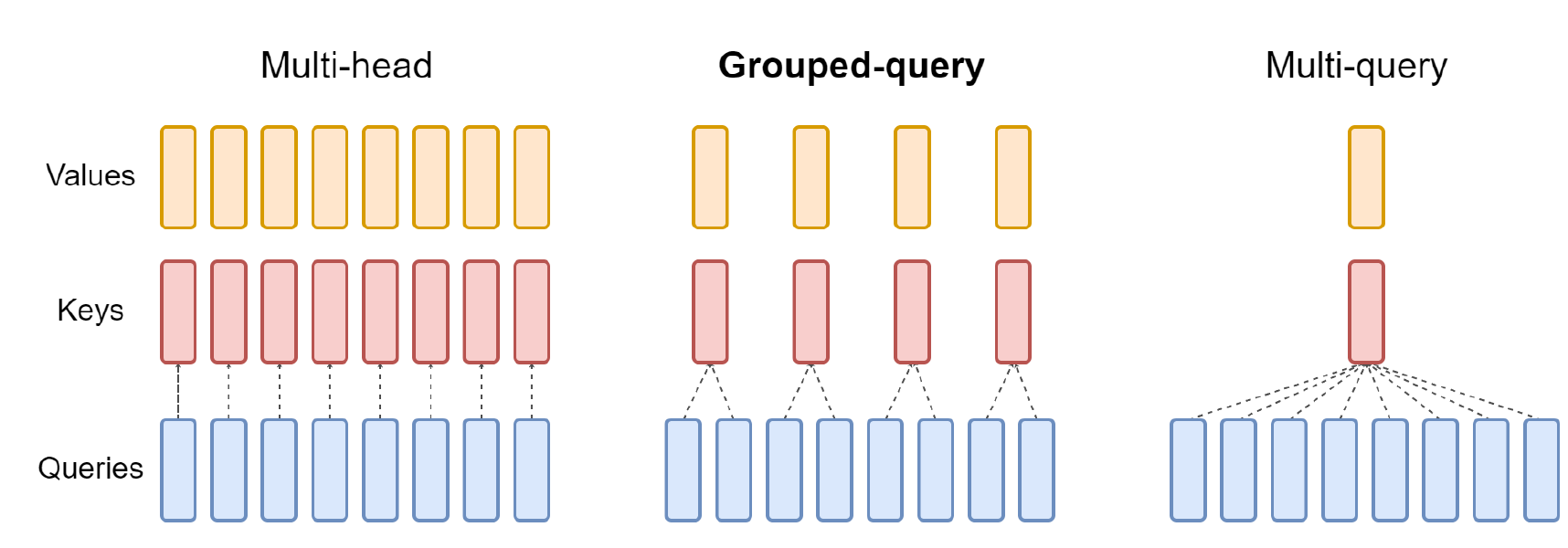
With groups, the cache holds key-value heads instead of one per query head: GQA-1 is MQA, and GQA- is ordinary multi-head attention.
Figure 2 from Ainslie et al. (2023), GQA: Training Generalized Multi-Query Transformer Models from Multi-Head Checkpoints · CC BY 4.0 · cropped, caption rewrittenThe cache shrinks by the ratio of query heads to key-value heads. Giving Llama 2 13B eight key-value heads instead of forty cuts its cache from 800 KiB to 160 KiB per token, and the model also shrinks a little, to 11.3 billion parameters, because the key and value projections shrink:
       8      1    22.7 GB     0.17 GB    22.8 GB     6.8 ms/token       147 tokens/s
       8     64    22.7 GB     0.17 GB    33.4 GB    10.0 ms/token     6,417 tokens/s
       8    256    22.7 GB     0.17 GB    65.6 GB    19.6 ms/token    13,068 tokens/s
At the same batch, GQA is faster and has higher throughput, because each step reads less; and the freed memory lets the batch grow to 256, which the original model could not hold. What it costs in quality depends on how the model was made:
- The GQA paper. Ainslie et al. converted T5-XXL, an encoder-decoder, from multi-head attention and uptrained it for 5% of its original pre-training compute. GQA-8 scored 47.1 on their benchmark average against 47.2 for multi-head, at 0.28 s per sample instead of 1.51 s.
- DeepSeek’s comparison from scratch. For the DeepSeek-V2 paper, DeepSeek trained three 7B dense models on the same 1.33T tokens, identical but for the attention (with layer counts adjusted to keep each near 7B parameters). On MMLU: 45.2 with multi-head, 41.2 with 8-group GQA and 37.9 with MQA.
Sharing heads is not free; it is cheap enough that nearly every recent open model does it. Qwen2.5-1.5B shares each key-value head among six query heads, which is why its cache is 28 KiB per token.
Compressing the cache: multi-head latent attention
DeepSeek-V2 (2024) took a different route. Multi-head latent attention (MLA) keeps all 128 of its key and value heads but never caches them. Each token’s hidden state is projected down to a small latent vector, only the latent is cached, and keys and values are projected back up from it when attention needs them:


Per token and layer, MLA caches 576 numbers where full multi-head attention with the same 128 heads would cache 32,768.
Drawn from Section 2.1 of DeepSeek-AI (2024), DeepSeek-V2: A Strong, Economical, and Efficient Mixture-of-Experts Language ModelTwo details make it work. The up-projection never has to run at inference: in the paper’s words, ” can be absorbed into , and can be absorbed into ”, so attention runs directly against the latents. That trick breaks under rotary position embeddings, because a position-dependent rotation would sit between the two matrices, so MLA carries position in a separate small key, rotated and shared by all heads, and caches that too. The sizes are the paper’s: a 512-dimensional latent plus a 64-dimensional rotary key, 576 numbers per token per layer against for multi-head attention, 57 times smaller; over DeepSeek-V2’s 60 layers, 67.5 KiB per token in 16-bit.
In the paper’s ablations (Table 9), DeepSeek trained pairs of mixture-of-experts models identical but for the attention. MLA scored slightly higher than multi-head attention on all four hard benchmarks at the large scale and on three of four at the small one, while caching 4% and 14% as much. The paper’s headline numbers for the deployed model, that it “reduces the KV cache by 93.3%, and boosts the maximum generation throughput to 5.76 times”, are measured against an older, different model, DeepSeek 67B, and the deployed server also quantizes its cache to about 6 bits per number, so they are not a measure of MLA alone.
Sharing across layers: cross-layer attention
Cross-layer attention (CLA, Brandon et al., 2024) lets adjacent layers share one set of keys and values: only some layers compute and cache their own, and the layers between reuse them.
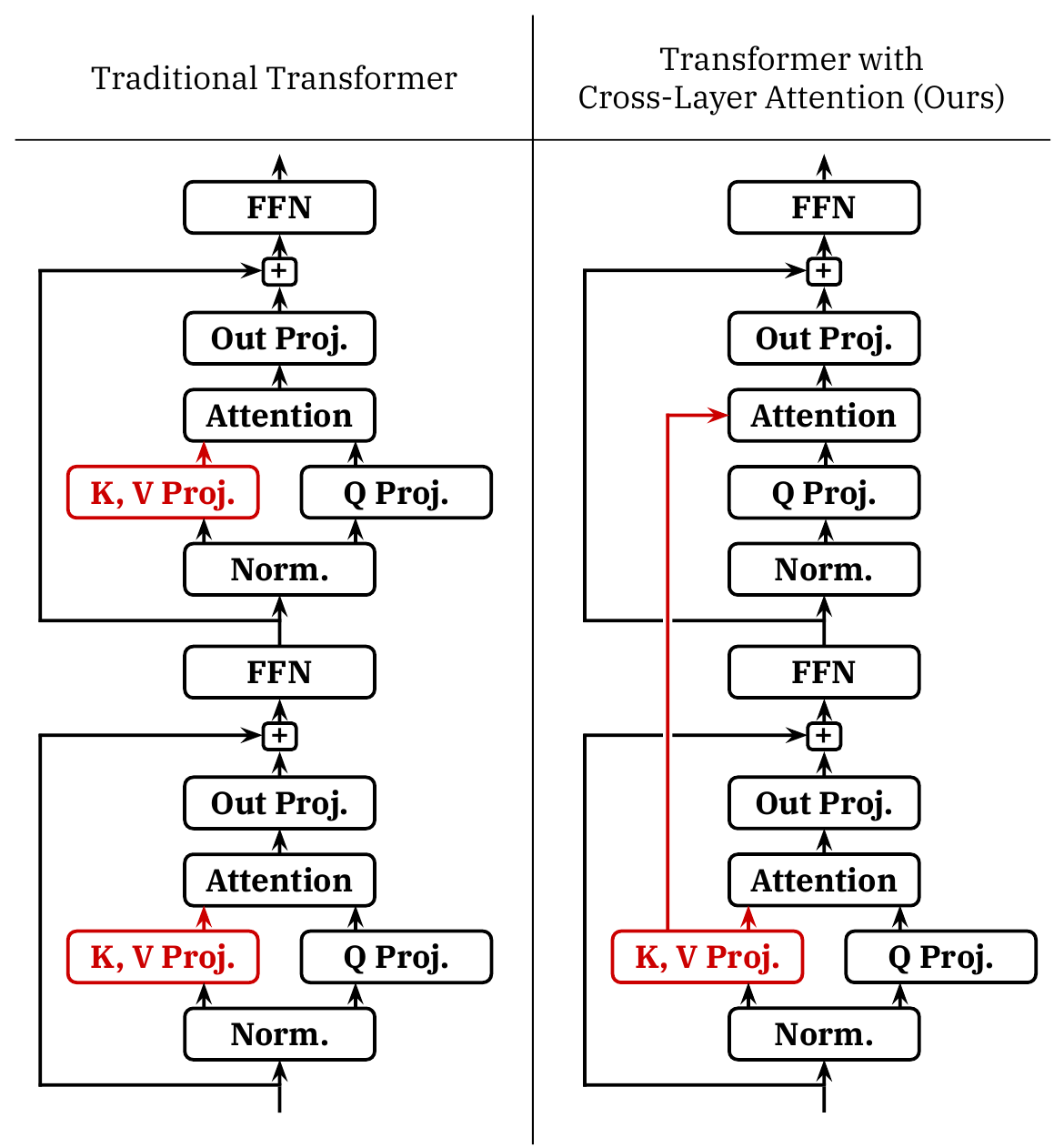
Left: every layer computes and caches its own keys and values. Right: the upper layer reuses the lower layer’s, so only one of the two is cached.
Figure 1 from Brandon et al. (2024), Reducing Transformer Key-Value Cache Size with Cross-Layer Attention · CC BY 4.0 · cropped, caption rewrittenSharing between pairs of layers (CLA2) halves the cache, and it stacks with MQA or GQA. In the authors’ 1B and 3B models trained from scratch, MQA plus CLA2 cut the cache “by another 2× while maintaining nearly the same accuracy as unmodified MQA”. The three ideas stack because they cut different factors of the formula: GQA and MQA reduce , CLA reduces the effective , and MLA replaces with one small latent.
What a naive cache does not solve
Two problems are about the cache’s shape, not its size.
Batching means padding, unless the cache is paged. A naive
implementation stores a batch’s cache as one tensor of shape [batch, max_len, ...], so every sequence is padded to the longest one, even after
it has finished. Paged Attention
breaks the cache into fixed-size blocks so that this padding disappears.
The cache is append-only, but serving is not. Everything above assumes tokens are only added at the end. Speculative Decoding, Derived proposes several tokens at once and rejects a suffix of them, whose keys and values must be removed before decoding continues; an agent that edits an earlier turn has the same problem at a coarser grain. A production cache has to truncate back to an earlier length, and share prefixes between requests (SGLang and RadixAttention).
Where this leads
- Paged Attention allocates the cache in fixed-size blocks, so no memory is lost to padding.
- Attention Alternatives stores fewer tokens: sliding windows keep only recent ones, and linear attention replaces the cache with a fixed-size state.
- KV Cache Compression stores each token in fewer bytes, by quantizing the cache or evicting tokens.
Takeaways
- Caching is exact: the projections are fixed and the causal mask means a later token can never change an earlier one’s keys or values. In Qwen2.5-1.5B-Instruct the cached and recomputed logits picked the same token after the prefill and at all 31 cached decode steps.
- Keys and values are cached, not queries: a query is used at one step, a key and value at every later step.
- The cache turns quadratic work into linear: at 4,096 tokens, one step took 65 ms with it and 4,727 ms without, on a laptop.
- The cache costs bytes per token, exactly: 28 KiB measured for Qwen2.5-1.5B; 512 KiB for Llama 2 7B.
- Decode is memory-bound: the MLP’s intensity is the batch size, and attention’s is below 1 whatever the batch. Batching raises throughput and latency together, and the batch is capped by cache memory: for Llama 2 13B on an H100, batch 64 gives about 22 times the throughput of batch 1 at 3 times the latency, and batch 256 does not fit.
- GQA, MLA and cross-layer attention shrink different factors of the formula, so they combine.
References
Start with kipply’s Transformer Inference Arithmetic and the Scaling Book’s inference chapter for the memory and intensity arithmetic, then the GQA and DeepSeek-V2 papers for how the cache is shrunk.
- kipply, Transformer Inference Arithmetic (2022): the cache’s memory formula and the compute- and memory-bound analysis.
- Austin et al., How To Scale Your Model: All About Transformer Inference (2025): the arithmetic intensity of prefill and decode, which the memory-bound section follows.
- Stanford CS336, Lecture 10: Inference (Spring 2026): the MLP and attention intensities and the Llama 2 13B latency and throughput model, recomputed here.
- Vaswani et al., Attention Is All You Need (NeurIPS 2017): the Transformer.
- Shazeer, Fast Transformer Decoding: One Write-Head is All You Need (2019): multi-query attention.
- Ainslie et al., GQA: Training Generalized Multi-Query Transformer Models from Multi-Head Checkpoints (EMNLP 2023): grouped-query attention, and the uptrained T5-XXL results.
- DeepSeek-AI, DeepSeek-V2: A Strong, Economical, and Efficient Mixture-of-Experts Language Model (2024): multi-head latent attention, decoupled RoPE, and the MHA/GQA/MQA/MLA ablations (Tables 8 and 9).
- Brandon et al., Reducing Transformer Key-Value Cache Size with Cross-Layer Attention (2024): sharing keys and values across adjacent layers.
- Kwon et al., Efficient Memory Management for Large Language Model Serving with PagedAttention (SOSP 2023): the paged KV cache.